Using the
date timing of intense Sporadic E Layer VHF radio reflections to forecast July,
summer and Early Autumn weather (temperature) trends by Dr Chris Barnes Bangor Scientific and
educational consultants e-mail manager@bsec-wales.co.uk May 2015.
Abstract
A new method for UK summertime temperature
anomaly prediction based on intense VHF sporadic E radio reflection is proposed
and validated. Temperature data prediction is available 1-2 months earlier than
using other methods.
Introduction
The phenomenon of Sporadic E radio reflection has
been known about for several decades now, in fact since as far back in history as
when high power VHF TV and FM
broadcasting began in the UK and USA and signals were often observed to be
received in very anomalous and none line of sight locations [1]. It has
also been understood that the phenomenon cannot take place unless there is
stratification in the E region of the ionosphere, see Whitehead (1990) [2].
Further, more and more is becoming understood
about this propagation mechanism and stratification. Because Sporadic E is related to multiple
triggers involving vertical shear of horizontal travelling ionisation waves in
the ionosphere initially of meteoric origin but strongly influenced by
planetary tides and waves, gravity waves from the atmosphere below including by
jet streams, thunder storms, earthquakes and volcanoes to name a few, I have
recently and somewhat remarkably been able to show a complex link between the
QBO ( Quasi –biennial Oscillation) of
the equatorial winds and the spring/
summer start dates of the sporadic E season. The relationship is a complex 4TH
order polynomial and similar complex
equations link UK monthly climate anomalies and QBO phase and descent rate, see
Barnes 2015 [3]. I have also
shown that similar equations hold for an entire season. Figure 1 shows the
polynomial equation which predicts the start of the sporadic E season as a
function of QBO phase and descent rate together with a compilation function QBO
with hindsight summer season temperature anomalies since 1980.
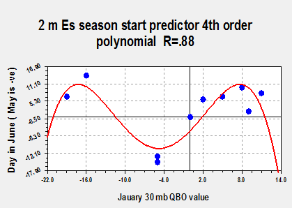
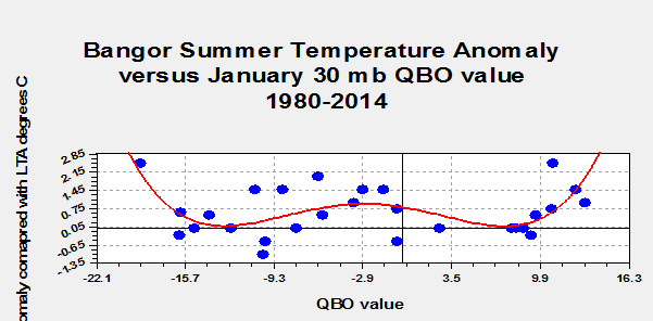
Figure 1 : Base polynomial equations showing QBO predicting both
retrospective 2m Es propagation and summer season
temperature.
Consider the P Value Results, firstly for the Es predictor:
We have, r=.88 DF=10
(10 degrees of freedom) thus the two-tailed P value equals 0.0002. By all conventional
criteria, this difference is considered to be extremely statistically
significant.
Further and secondly consider the P Value Results for the summer
temperature anomaly : P Value Results r=.563
DF=28 ( 28 degrees of freedom)
Here, the two-tailed P value equals
0.0012 by conventional criteria, this difference is also considered to be very
statistically significant.
Interestingly the residuals are far greater
with negative QBO and there are almost two distinct bands to the data between
QBO 0 and -16 which may be solar/NAO/AO effects. I have discussed these elsewhere [4].
Effectively, separate start dates can be defined
according to MUF (maximum useable frequency).
As far as investigation by radio amateurs is concerned their use of
frequency is constrained to the various operating bands which their license
permits them to use. For instance the
VHF bands are the 6m band (50-54 MHz), available in all European and American
countries, the 4m band (70-70.5 MHz) only available in certain countries and
the 2m band ( 144-148 MHz) available in all countries. Basically the higher the frequency band,
the higher needs to be the MUF in order to access the Sporadic E mode of radio
reflection/propagation. Since far more
intense ionisation is required at the highest MUF’S these type of conditions
only occur about 4-8 times per annum and usually later than the start date as
defined for lower MUF’S.
Typically the
6m spring/summer Es season commences in April but the 2m season
not until May, June or even July.
Hypothesis
Since both climate anomaly and Sporadic E event
dates have been shown to correlate with QBO through sets of polynomial
equations there ought also to be some sort of correlation between climate
anomaly and sporadic E dates.
Furthermore, the significant features of the two polynomials as plotted
above , figure 1, appear to be mirrored across the abscissa or at least
approximately mirrored, suggesting that when one function is divided by the other a significant degree of linearization ought to take
place.
Experimental
The start of the Sporadic E season is actually quite
hard to define as occurrences at lower MUFS
can be very common. It was decided therefore to define the start of the
2m ( 144 MHz) season instead and also because using hindsight data from radio communication journals it is expected to be far better
documented. Since the Es clouds drift in time and space it is necessary to define a geographical
area for each event. The author is interested in the UK climate, especially
Wales. Generally sizeable sporadic E
events affecting the UK will also effect Wales and Eire.
Only the earliest 2m events effecting these
countries at one end of a propagation path were considered in choosing dates to
define the first significant event of each year in the study.
The climate anomaly data sets were available at the
UK met office website [5, 6].
The first and earliest significant 2m events usually take place in May
or June and very occasionally July. It was thus decided to see if the dates of these
events could be used in hindsight prediction of July, Summer
and Early Autumn temperature anomaly.
The results were plotted using a well-known
graph package, namely Curve Expert by Hyams [7].
The statistical significance ( p-values) were
obtained using an on –line calculator
from the Regression factors and number of degrees of freedom. The data set sought after was
1976-2014. However, since amateur radio
data has not been stored on the internet for very long, data regarding 2m
Sporadic E events was very sparse in all but the later few of these years,
accounting for the differing numbers of degrees of freedom, figure 1. Furthermore, the UK climate anomaly is differently recorded by the Met Office for different
years. In the years 2001 – 2015,
graphical and tabulated numeric data is available [5]. However, before 2001 only GIS style mapping
is available with a significant
deterioration in accuracy [6].
Results
and Discussion
Figure 2 shows the result for the Bangor area of
Gwynedd and data taken from the GIS maps.
Summer temperature anomaly refers to the average for all three summer
months June-August inclusive.
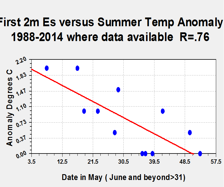
Figure 2
The regression factor of .76 with 12 degrees of freedom is highly statiscally significant, with
p= 0.0016
Figure 3 shows the method exteneded
for the whole of Wales and using the more accurate, 2001- 2014 dataset.
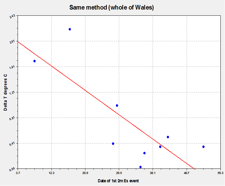
Figure 3:
R=.79
Further
regressions were attempted for the months of July, August and September
separately. A regression factor of .78
was obtained for July, no correlation for August and a factor of .57 (p=.033)
for September.
It is thus possible to use the method to predict
temperature anomaly for July with some considerable certainty and for the whole
of the summer and for the early autumn period but not for August which in North
Wales appears to be a most unpredictable month.
Once again ‘banding’ in the residuals is seen which
may be inherited from the – ve QBO data and is
possibly the only thing that limits this technique.
An independent test of this was to consider if
hindsight July temperatures could be used to make similar predictions. It was
shown that July could predict September temperatures with reasonable
certainty but not August. Yet both strangely
and similarly to the case with the Sporadic E method predictor July
temperatures are an excellent predictor of the averaged anomaly spread across
both August and September, see Figure 4.
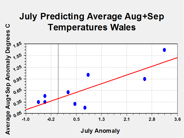
Figure 4,
Hindsight prediction of August + September from July anomaly, R=.81
The Sporadic E method is further justified by
comparing the monthly regression factors like against like, figure 5.
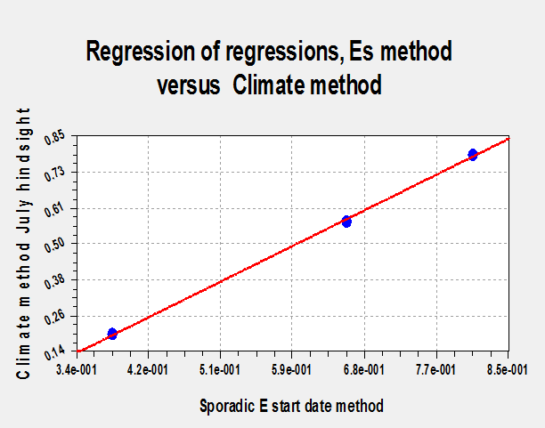
Figure 5
Let us consider the P Value Results. We have r=.99963 DF=3
giving a two-tailed P value is
less than 0.0001, considered to be extremely statistically significant.
In other words the sporadic E 2m start date method
has been proved to be a valid climate anomaly prediction method for North Wales
Summer Climate temperature anomaly.
Further
discussion
It is clear the initial hypothesis is strongly supported and validated from the
point of view of mathematical analysis, but what evidence is there for its physical
basis?
Intense sporadic E openings have long been associated
with severe thunderstorms. From personal
research I have found jet stream orientation and thunderstorms together are
quite critical for the propagation mode.
Davis and Johnson (2005) [8]
have emphasized the notion of
Lightning-induced intensification of the ionosphere sporadic E layer. It has been proposed, on the basis of a few observed
events that the ionospheric 'sporadic E'
layer—transient, localized patches of relatively high electron density in the
mid-ionosphere E layer, which significantly affect radio-wave propagation—can
be modulated by thunderstorms. They identified a statistically significant
intensification and descent in altitude of the mid-latitude sporadic E layer
directly above thunderstorms. Because no ionospheric
response to low-pressure systems without lightning was detected, they concluded
that this localized intensification of the sporadic E layer can be attributed
to lightning. They suggested that the co-location of lightning and ionospheric enhancement could be explained by either
vertically propagating gravity waves that transfer energy from the site of
lightning into the ionosphere, or vertical electrical discharge, or by a
combination of these two mechanisms.
Lightning data, collected using a Boltek Storm Tracker system installed at Chilton, UK, were
used to investigate the mean response of the ionospheric
sporadic-E layer to lightning strokes in a superposed epoch study. This
lightning detector can discriminate between positive and negative lightning
strokes and between cloud-to-ground ( CG) and
inter-cloud ( IC) lightning. Superposed epoch studies carried out separately
using these subsets of lightning strokes as trigger events have revealed that
the dominant cause of the observed ionospheric
enhancement in the Es layer is negative
cloud-to-ground lightning. In my opinion, this would help account for why
not every single thunderstorm causes a sporadic E radio propagation event.
Whitehead (1988) has suggested that Mid-latitude sporadic-E is most likely
due to a vertical shear in the horizontal east-west wind and this theory
accounts for the detailed observations of the wind and electron density
profiles. Preferred heights of sporadic-E are separated by about 6km and
descending layers are often seen moving down with velocities in the range 0.6–4
ms−1. Sometimes sporadic-E layers are very flat and uniform, and at other
times form clouds of electrons 2–100km in size moving horizontally at 20–130 ms−1.
Sporadic-E is probably not correlated with meteor showers; this is a rather
surprising result since the ions are meteor debris. However, meteoric debris has a very long lifetime
in the atmosphere [9].
Vertically propagating gravity waves from storms can
provide Whitehead’s shear. Sprites have
been identified as evidence of vertical gravity wave structures above mesoscale
thunderstorms. Large area multicell
thunderstorms lead to the formation of vertically oriented cylindrical
structures of gravity waves at mesospheric altitudes closely resembling those
observed in optical emissions associated with transient luminous glows called
sprites. Taylor (1988) observed
a short period gravity wave train was detected by its
effect on three upper atmospheric nightglow emissions, the OI 557.7 nm and Na
589.2 nm lines and the OH bands between 715 and 810 nm (Taylor et al., 1987,
Planet. Space Sci. 35, 413). Images of these emissions, which were recorded on
the evening of 14 August 1980 from the Gornergrat
Observatory, Switzerland (45.98°N, 7.78°E), contained high contrast wave-like
structures coherent in all three emissions and exhibiting curvature. These
properties have been used to identify a thunderstorm centred over southern
France as the most likely source of the waves. Interestingly, Es clouds are known for their curved surfaces ideal for
radio reflection.
Woodman et al has further elucidated the Es process, finding that wave-like features in range seen
on the range/time/intensity (RTI) records of VHF backscatter radars operating
in the South of New Zealand are interpreted as being the signature of gravity waves
propagating in an ionospheric sporadic-E layer. The
data show that, during midsummer in particular, sporadic-E ionisation which has
been modified by the passage of a gravity wave can produce two distinct echo types:
backscatter from field-aligned irregularities within the sporadic-E layer,
probably generated by plasma waves, and a second type of echo resulting from
energy backscattered from the surface of the sea after specular reflection in
the ionosphere. The backscattering and reflecting region can exist at latitudes
at least as low as 49° geographic (57° geomagnetic) latitude during quiet
magnetic conditions. They confirmed the patchiness of dense sporadic-E, and
concluded that gravity waves at sporadic-E heights have amplitudes of the order
of several tenths of a kilometre. They
also concluded that more than likely only Gravity waves with phase fronts parallel
to the magnetic dip angle were capable of producing such distortion in
a normally stable and radio inactive E layer , imposing its own temporal and
spatial periodicity on the echoes. This probably
additionally accounts for why not all thunderstorms produce sporadic E. By my own personal experience I have found
that thunderstorms tend to be more effective towards the south of an east-west
radio propagation path and can sometimes be as much as 200 km south of that
path. Only once have I experienced intense
2m E’s propagation centrally in a UK thunderstorm.
Fritts and Nastrom.(1992) [10]
considered four cases of mesoscale variance enhancements of horizontal velocity
and temperature due to frontal activity, non-frontal convection, and wind shear.
These data were obtained aboard commercial aircraft during the Global
Atmospheric Sampling Program (GASP) in 1978 and 1979 and from the corresponding
meteorological analyses and satellite imagery. Additional GASP data were used
to permit a statistical assessment of the importance of various sources of
enhanced variances. The results, and those in their companion paper addressing
the variance enhancements associated with topography, represent refinements of
previous source analyses using the GASP dataset. Significant findings include
mean variance enhancements of velocity and temperature due to convection and
jet-stream flow ranging from ∼2 to 8 for 64-km and 256-km data segments, and
enhancements for individual segments as high as ∼20
to 100. The mean 64-km variance enhancement for all variables and source types,
relative to a quiescent background, was estimated to be 6.1. These results
suggest a major role for localized sources in energizing the mesoscale motion
spectrum at horizontal scales < ∼100
km, and correspondingly greater influences for such motions at greater heights.
KH billows similar to those found in the
troposphere are also found in the E-layer.
Others have shown theoretically that modulation of
electron densities in ion layers between 90 and 110 km altitude has been observed using a
number of ionospheric diagnostic measurements
including scatter of VHF radar waves, artificially pumped optical emissions,
scintillations of satellite beacon transmissions. Kelvin–Helmholtz (K–H) turbulence
driven by a sheared wind profile is a strong candidate for the source of these
modulations. A two-dimensional numerical model is used to calculate the
nonlinear evolution of ion layers in ionosphere near 100 and altitude in
response to neutral turbulence driven by a wind shear. The amplitude of a K–H
billow is allowed to grow as a linear perturbation on the neutral atmosphere to
a level that is 10% of the wind shear. The time dependent model of the
ionosphere responds to neutral wind perturbation initially by imposing a
quasi-sinusoidal modulation near the altitude of the ion layer. This is
followed by compression of the initially stratified layer into structures with
the wavelength of the K–H instability. These structures are uniform strips in
the meridian perpendicular to the direction of the zonal wind. Near, where the
ion gyro frequency (ωi) is about equal to the
ion collision frequency, the equilibrium solutions are clumps at the altitude
of the shear. Near, two stable, rippled layers are produced with a given separation.
The amplitudes of the density modulations in the ion layers vary by as much as
500% throughout the simulation. The simulations illustrate the complex
evolution of the ion layer structures from small-amplitude, K–H wind turbulence.
Existing theory of the stability of a stably
stratified fluid containing a strong vertical shear suggests that unstable
waves may develop when the curvature of the velocity profile changes sign and
the Richardson number is somewhere less than 1/4. Some observations are
described which show the properties of atmospheric billow clouds formed in
travelling amplifying waves (transverse to the shear vector), on occasions when
these conditions appear to be met. Static instability seems to arise in parts
of the wave-pattern where layers are inverted, and to cause a convective
overturning, which may halt the wave development. The most pronounced waves
occur in the upper troposphere in association with jet streams, in layers of
strong wind shear which are usually dry. They probably only rarely produce
clouds, and may more frequently be responsible for the clear-air turbulence
encountered by aircraft. The associated relative air velocities occur over a
range of scales: up to about 1 km in the convective regions, and up to the
several km associated with the billow wave-lengths, with magnitudes of up to 10
m sec−1 or more. Of course jet
streams are another E’s trigger long since acknowledged by radio hams. Clearly
their upwardly propagating billow initiated gravity waves are essential as
thunderstorms.
Such billows are found in reality by analyzing the field-aligned coherent radar backscatter
observed, for example, this was done over Gadanki,
India (13.5°N, 79.2°E), with a narrow beam pointing almost vertically, Choudhary et al (2005) [11] present convincing
experimental evidence for the presence of low-latitudes tilted sporadic
ionization layers close to 10 km in vertical extent that move horizontally
through the field of view of the radar. Using the data from high temporal (∼3 s) resolution experiments, we also show that the
line-of-sight Doppler velocities associated with at least some of the
quasi-periodic striations have very clear vortex-like structures cutting across
a vertical plane inside regions of strong horizontal wind shears. The power as
well as the Doppler width peak together, and they often reach their peak values
near the centre of a vortex, where the magnitude of the Doppler velocity is
minimum. The Doppler properties and spatial distribution of the 3 m echoes are
explained in terms of a local electro dynamical process that makes ions and
electrons move with the vertical neutral wind. Both the wind field and the tilt
of the layers are in turn consistent with the presence of Kelvin-Helmholtz
billows. Billows themselves are triggered by a shear instability in the large
ambient zonal wind; strong zonal wind shears clearly have to be present when
sporadic E layers are observed. In our case, the breaking of an originally
uniform and horizontal sporadic E layer into tilted pieces aligned more or less
parallel to one another, and their motion through the radar field of view in
the presence of a mean zonal wind, give the echoes their quasi-periodic
appearance. Here the link between QBO
and E’s is re-affirmed.
Let us re-visit lighting. In a warmer climate more
lightning is to be expected. Price and Rind (1994) and Price (2008) [12]
have made the analysis. They use the
Goddard Institute for Space Studies (GISS) general circulation model (GCM) to
study the possible implications of past and future climate change on global
lightning frequencies. Two climate change experiments were conducted: one for a
2×CO2 climate (representing a 4.2°C global warming) and one for a 2% decrease
in the solar constant (representing a 5.9°C global cooling). The results
suggest a 30% increase in global lightning activity for the warmer climate and
a 24% decrease in global lightning activity for the colder climate. This implies an approximate 5–6%
change in global lightning frequencies for every 1°C global warming/cooling.
Both intra-cloud and cloud-to-ground frequencies are modelled, with
cloud-to-ground lightning frequencies showing larger sensitivity to climate
change than intra-cloud frequencies. The magnitude of the modelled lightning
changes depends on season, location, and even time of day. The notion of increased cloud to ground
lightening is particularly relevant to the case in hand, we have already seen
above it is negative cloud to ground lightening which has been associated with
sporadic E enhancement.
It is instructive to consider the behaviour of
lightning in Europe, see Figure 6 below.
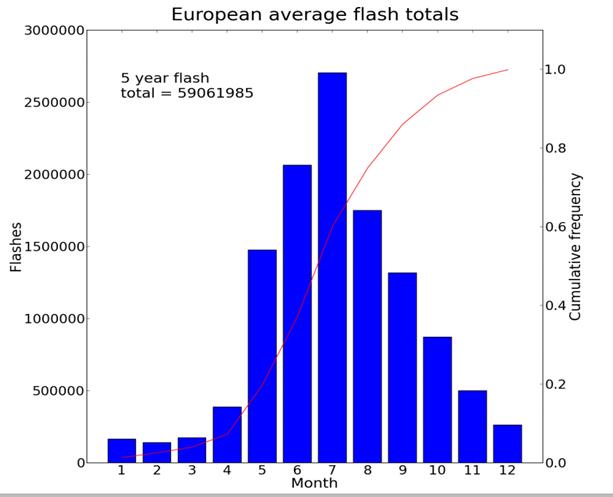
eFigure 6
The peak month for commencement of the 2m Es season is June.
The average date for commencement is June 3rd. Thus we may regard this date as being
related to 10% of the duration of this month can be regarded as having a 10%
increase in flashes over May assuming linearity in the cumulative frequency
slope. The highest positive anomaly within the period was 2.6 C and the lowest
negative anomaly was -0.5 C. Based on
Price and Rind’s calculation, 3.2 C represents a 19.2 day advancement of the
start to the season i.e. circa May 14th. A .5 C negative anomaly represents a 2 day
retardation. In the real data set for North Wales, the largest advancement in
2m Es season start date noted was some 26 days and the
largest retardation was some 18 days. Thus the hypothesis that summer climate temperature
prediction by following E’s start date as a result of earlier temperature enhanced lightening activity is strongly
supported.
Possibly some other factor could also be at work. Rishbeth (1990) [13]
has considered the possibility of a greenhouse effect in the ionosphere. Following a suggestion by Roble and
Dickinson that increases in the mixing ratios of mesospheric carbon dioxide and
methane will cool the thermosphere by about 50K, their paper examines the
consequences for the ionosphere. The cooling and the associated composition
changes, as described by Roble and Dickinson, would lower the E- and F2-layer
peaks by about 2 km and 20 km respectively, but changes in the E- and F2-layer
electron density are small. It is uncertain
if such small height changes in the E layer prior to stratification would be
sufficient to changes E’s start date significantly.
In any event at least for the moment, anthropogenic
changes do not seem to have invalidated the method.
Further
work
It is hoped to investigate the relationship between
Sporadic E and rainfall in another publication in due course.
Conclusions
A new method for UK summertime temperature anomaly
prediction based on VHF sporadic E radio reflection has been proposed and validated.
Although marginally less accurate than using July temperature data prediction
is available 1-2 months earlier.
References
1.
http://en.wikipedia.org/wiki/TV_and_FM_DX#History
2.
http://www.sciencedirect.com/science/article/pii/027311779090013P
3.
RadCom Plus,
Vol. 1, No. 1 pp 22-30 May 2015 http://rsgb.org/main/blog/front-page-news/2015/04/30/radcom-plus-vol-1-1/
4.
http://www.drchrisbarnes.co.uk/CLI.htm
5.
http://www.metoffice.gov.uk/climate/uk/summaries/anomalygraphs
6.
http://www.metoffice.gov.uk/public/weather/climate-anomalies/#?tab=climateAnomalies
7.
http://www.curveexpert.net/download/
8.
http://www.nature.com/nature/journal/v435/n7043/abs/nature03638.html
10. http://ntrs.nasa.gov/search.jsp?R=19920041497
11. http://onlinelibrary.wiley.com/doi/10.1029/2004JA010987/full
12. http://www.iclp-centre.org/pdf/Invited-Lecture-1.pdf
13. http://www.sciencedirect.com/science/article/pii/003206339090061T